![]()
Relational Group Activity Recognition
Table of Contents
Key Updates
- ResNet-50 Backbone: Replaced VGG19 with ResNet-50 for stronger feature extraction.
- Ablation Studies: Comprehensive experiments to evaluate the contribution of each model component.
- Test-Time Augmentation (TTA): Implemented to improve robustness and reliability during inference.
- Graph Attention Operator: Implementation for an attention-based relational layer.
- Improved Performance: Achieves consistently higher accuracy across all baselines compared to the original paper.
- Modern Implementation: Fully implemented in PyTorch with support from PyTorch Geometric.
Introduction
Traditional pooling methods (max, average, or attention pooling) reduce dimensionality but often discard important spatial and relational details between people. The Hierarchical Relational Network (HRN) addresses this by introducing a relational layer that explicitly models interactions between individuals in a structured relationship graph.
How the Relational Layer Works
Graph Construction
- Each person in a frame is represented as a node.
- People are ordered based on the top-left corner
(x, y)of their bounding boxes (first by x, then by y if tied). - Edges connect a person to their neighbors, forming cliques in the graph.
Initial Person Features
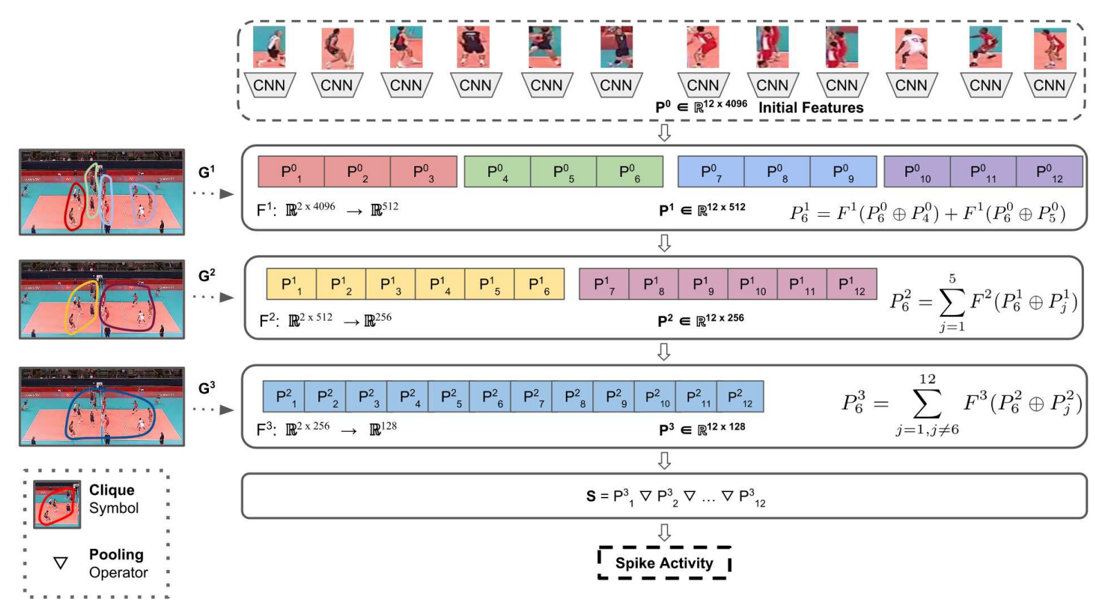
Each person’s initial representation comes from a CNN backbone (e.g., ResNet50):$$P_i^0 = \text{CNN}(I_i)$$
where $I_i$ is the cropped image around person $i$.
Relational Update
At relational layer $\ell$, person $i$’s updated representation is:
$$P_i^\ell = \sum_{j \in E_i^\ell} F^\ell(P_i^{\ell-1} \oplus P_j^{\ell-1}; \theta^\ell)$$
- $E_i^\ell$: neighbors of person $i$ in graph $G^\ell$
- $\oplus$: concatenation operator
- $F^\ell$: shared MLP for layer $\ell$ (input size $2N_{\ell-1}$, output size $N_\ell$)
- This step computes pairwise relation vectors between $i$ and its neighbors, then aggregates them.
Hierarchical Stacking
- Multiple relational layers are stacked, compressing person features while refining relational context.
- The architecture supports a variable number of people $K$ (robust to occlusions or false detections).
Scene Representation
The final scene feature $S$ is obtained by pooling person features from the last relational layer:$$S = P_1^L \ ▽ \ P_2^L \ ▽ \dots \ ▽ \ P_K^L$$
where $▽$ is a pooling operator (e.g., concatenation or element-wise max pooling).
Usage
1. Clone the Repository
| |
2. Install the Required Dependencies
| |
3. Download the Model Checkpoint
This is a manual step that involves downloading the model checkpoint files.
Option 1: Use Python Code
Replace the modeling folder with the downloaded folder:
| |
Option 2: Download Directly
Browse and download the specific checkpoint from Kaggle:
Relational-Group-Activity-Recognition - PyTorch Checkpoint
Dataset Overview
The dataset was created using publicly available YouTube volleyball videos. The authors annotated 4,830 frames from 55 videos, categorizing player actions into 9 labels and team activities into 8 labels.
Example Annotations
- Figure: A frame labeled as “Left Spike,” with bounding boxes around each player, demonstrating team activity annotations.
Train-Test Split
- Training Set: 3,493 frames
- Testing Set: 1,337 frames
Dataset Statistics
Group Activity Labels
| Group Activity Class | Instances |
|---|---|
| Right set | 644 |
| Right spike | 623 |
| Right pass | 801 |
| Right winpoint | 295 |
| Left winpoint | 367 |
| Left pass | 826 |
| Left spike | 642 |
| Left set | 633 |
Player Action Labels
| Action Class | Instances |
|---|---|
| Waiting | 3,601 |
| Setting | 1,332 |
| Digging | 2,333 |
| Falling | 1,241 |
| Spiking | 1,216 |
| Blocking | 2,458 |
| Jumping | 341 |
| Moving | 5,121 |
| Standing | 38,696 |
Dataset Organization
- Videos: 55, each assigned a unique ID (0–54).
- Train Videos: 1, 3, 6, 7, 10, 13, 15, 16, 18, 22, 23, 31, 32, 36, 38, 39, 40, 41, 42, 48, 50, 52, 53, 54.
- Validation Videos: 0, 2, 8, 12, 17, 19, 24, 26, 27, 28, 30, 33, 46, 49, 51.
- Test Videos: 4, 5, 9, 11, 14, 20, 21, 25, 29, 34, 35, 37, 43, 44, 45, 47.
Dataset Download Instructions
- Enable Kaggle’s public API. Follow the guide here: Kaggle API Documentation.
- Use the provided shell script:
| |
For further information about dataset, you can check out the paper author’s repository:
link
Ablation Study
Baselines
Single Frame Models:
B1-NoRelations: In the first stage, Resnet50 is fine-tuned and a person is represented with 2048-d features. In the second stage, each person is connected to a shared dense layer of 128 features. The person representations (each of length 128 features) are then pooled and fed to a softmax layer for group activity classification.
RCRG-1R-1C: Pretrained Resnet50 network is fine-tuned and a person is represented with 2048-d features, then a single relational layer (1R), all people in 1 clique (1C), so all-pairs relationships are learned.
RCRG-1R-1C-!tuned: Same as previous variant, but Pretrained Resnet50 network without fine-tuning.
RCRG-2R-11C: Close to the RCRG-1R-1C variant, but uses 2 relational layers (2R) of sizes 256 and 128. The graphs of these 2 layers are 1 clique (11C) of all people. This variant and the next ones explore stacking layers with different graph structures.
RCRG-2R-21C: Same as the previous model, but the first layer has 2 cliques, one per team. The second layer is all-pairs relations (1C).
RCRG-3R-421C: There relational layers (of sizes 512, 256, and 128) with clique sizes of the layers set to (4, 2, 1). The first layer has 4 cliques, with each team divided into 2 cliques.
Performance comparison
Original Paper Baselines Score
My Scores (Accuracy)
| Model | Test Acc | Test Acc TTA (4) | Paper Test ACC |
|---|---|---|---|
| B1-no-relations | 89.07% | 89.06% | 85.1% |
| RCRG-1R-1C | 89.42% | - | 86.5% |
| RCRG-1R-1C-untuned | 80.86% | - | 75.4% |
| RCRG-2R-11C | 89.15% | - | 86.1% |
| RCRG-2R-21C | 89.49% | - | 87.2% |
| RCRG-3R-421C | 88.97% | - | 86.4% |
| RCRG-2R-11C-conc | 89.60% | 89.71% | 88.3% |
| RCRG-2R-21C-conc | 89.60% | 89.60% | 86.7% |
| RCRG-3R-421C-conc | 89.23% | - | 87.3% |
Notes:
-concpostfix is used to indicate concatenation pooling instead of max-pooling.- Used 4 transform augmentation at TTA.
Temporal Models:
RCRG-2R-11C-conc-temporal: Uses 2 relational layers (2R) of sizes 256 and 128. The graphs of these 2 layers are 1 clique (11C) of all people.
RCRG-2R-21C: The first layer has 2 cliques, one per team. The second layer is all-pairs relations (1C).
Performance comparison
Original Paper Baselines Score
My Scores (Accuracy)
| Model | Test Acc | Test Acc TTA (3) | Paper Test ACC |
|---|---|---|---|
| B1-no-relations-temporal | 88.93% | 89.60% | - |
| RCRG-2R-11C-conc-V1 | 90.50% | 90.73% | 89.5% |
| RCRG-2R-11C-conc-V2 | 91.55% | 91.62% | 89.5% |
| RCRG-2R-11C-conc-V3 | 91.40% | 91.77% | 89.5% |
| RCRG-2R-21C | - | - | 89.4% |
Notes:
Temporal: postfix is used to indicate model work with a sequence of frames, not a frame.-concpostfix is used to indicate concatenation pooling instead of max-pooling.- The original paper did not clearly specify where the LSTM unit should be integrated into the model.
To explore this, I implemented three possible variants:V1: LSTM before the relational layer → allows the relational layer to learn richer spatio-temporal features.V2: LSTM after the relational layer → enhances the relational features with temporal modeling.V3: LSTMs both before and after the relational layer → combines the strengths of V1 and V2.
- I decided to train
RCRG-2R-11C-conconly, since it achieved the best performance in both my implementation and the paper’s results. - I implemented
B1-no-relations-temporalto evaluate the impact of the relational layer (This model was not included in the original paper).
Attention Models (new baseline):
- Uses 2 relational layers (2R). The graphs of these two layers are one clique (11C) of all players, but this time using a graph attentional operator instead of an MLP for the relational layers.
My Scores (Accuracy)
| Model | Test Acc | Test Acc TTA (3) | Paper Test ACC |
|---|---|---|---|
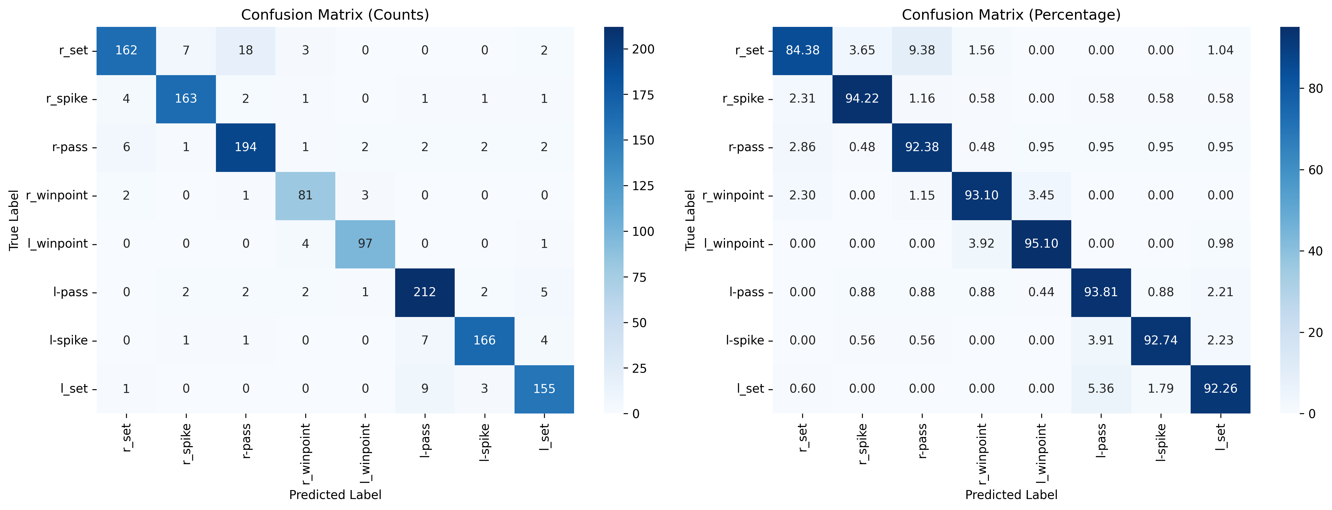
| RCRG-2R-11C-conc-V1 | 91.77% | 92.00% | - |
RCRG-2R-11C-conc-V1-Attention Confusion Matrix