DETR Architecture Components
Backbone for Feature Extraction 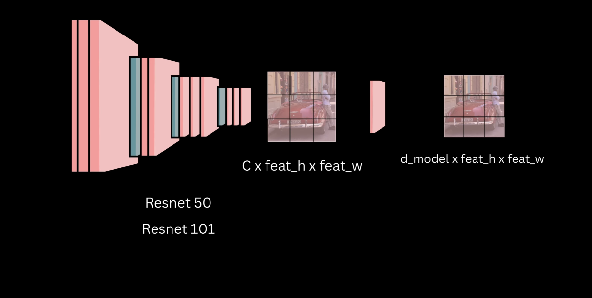
The initial input image is processed by a backbone, typically a pre-trained Convolutional Neural Network (CNN), such as ResNet 50 or ResNet 101, trained on the ImageNet classification task.
The last pooling and classification layers are discarded to produce a feature map that captures semantic information for different regions of the image.
The network stride is typically 32. The feature map output dimensions are $C \times \text{feature map height} \times \text{feature map width}$, where $C$ is the number of output channels of the last convolution layer.
A projection layer, implemented as a $1 \times 1$ convolution, is applied to transform the feature map dimensions. This step aligns the input channels with the backbone output and the output channels with the hidden dimension of the transformer, $D_{\text{model}}$. The resulting shape is $D_{\text{model}} \times \text{feature map height} \times \text{feature map width}$.
Transformer Encoder 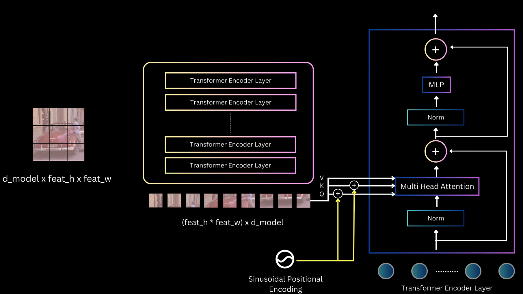
The projected feature map is flattened by collapsing the spatial dimensions, creating a sequence of $D$-dimensional features that serves as input to the encoder.
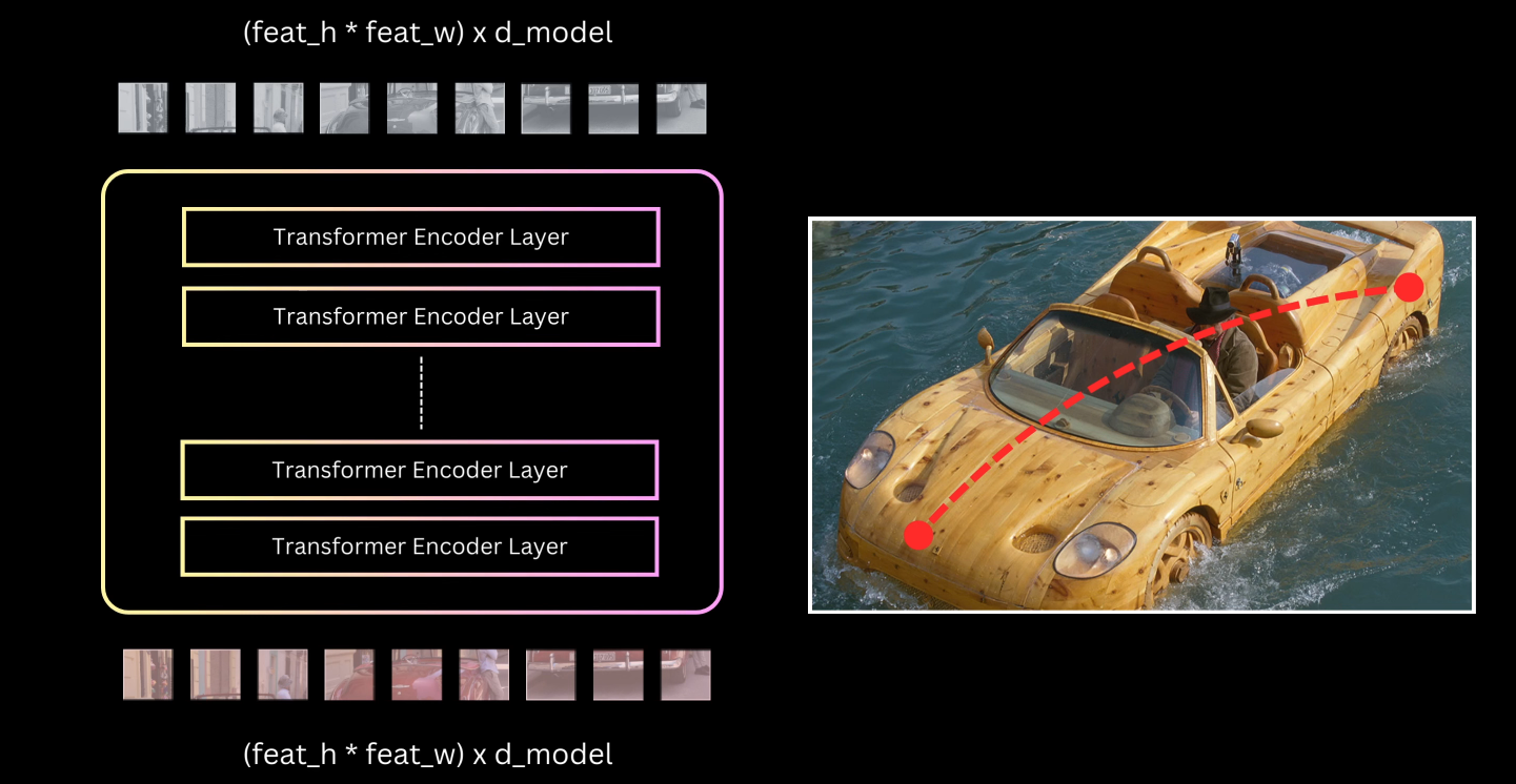
The encoder is a stack of transformer encoder layers, each consisting of self-attention and feed-forward layers, integrated with residual connections and normalization steps.
Through self-attention, the encoder transforms the backbone features into representations conducive for the detection task, establishing relationships between distinct image parts and baking in contextual knowledge.
Positional Encoding
Due to the permutation invariant nature of transformers, spatial positional information must be injected.
The original transformer’s sinusoidal position encoding is adapted for 2D images.
The D-dimensional position encoding for a spatial feature is created by concatenating $D/2$ dimensional encodings for the height coordinates and $D/2$ dimensional encodings for the width coordinates.
Unlike typical transformer usage, this positional information is added at each self-attention layer, specifically to the query ($Q$) and key ($K$) tensors, rather than just once at the input.
Transformer Decoder and Object Queries
The decoder requires two inputs: the transformed image features returned by the encoder, and $N$ object queries.
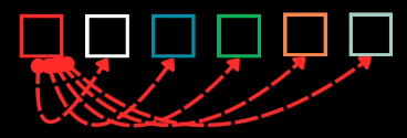
Object queries are $N$ randomly initialized, learnable embeddings that act as “slots” or containers which the model transforms to produce object predictions. The number of predictions equals the number of queries.
The decoder is a sequence of layers containing self-attention, cross-attention, MLP, normalization, and residual connections.
Self-Attention in Decoder: Enables queries to interact with each other, allowing the model to reason about all objects together using pair-wise relationships.
- The $N$ slots are typically initialized to zero, and $N$ embedding values, termed output position encoding, are added to the slots prior to computing $Q$ and $K$ representations within the attention mechanism.
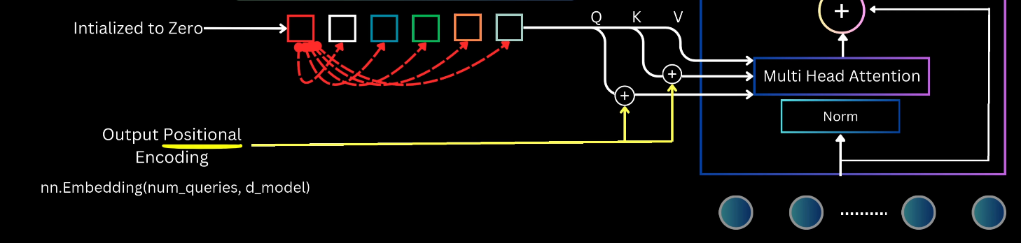
- The $N$ slots are typically initialized to zero, and $N$ embedding values, termed output position encoding, are added to the slots prior to computing $Q$ and $K$ representations within the attention mechanism.
Cross-Attention: Allows object queries access to the entire image context by attending to the features returned by the encoder.
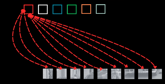
- The object queries form the $Q$ input, while the encoder image features form the $K$ and $V$ inputs.
- Positional information is added at each cross-attention layer: fixed sinusoidal positional embeddings are added to image features (prior to $K$ computation), and output position embeddings are added to slot representations (prior to $Q$ computation).
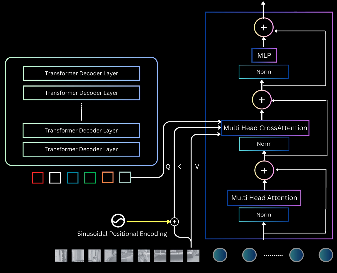
Prediction Heads: The $N$ output vectors from the final decoder layer are decoded independently into $N$ object predictions using two parallel MLPs whose parameters are shared across all query slots.
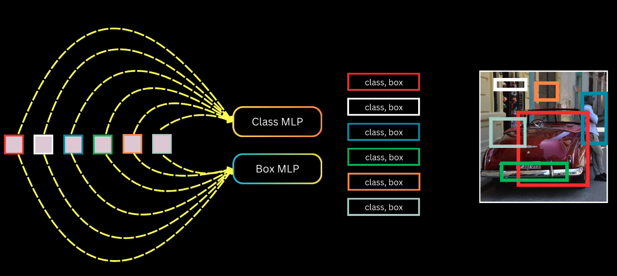
- A class MLP outputs class probabilities for the predicted box.
- A bounding box MLP outputs four normalized coordinates ($c_x, c_y, w, h$).
Set Prediction and Optimal Assignment
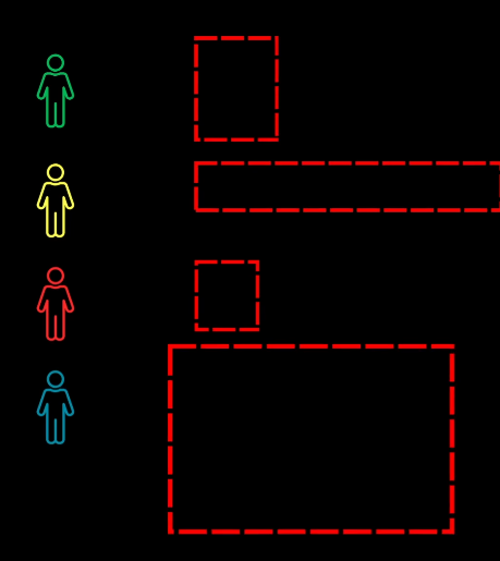
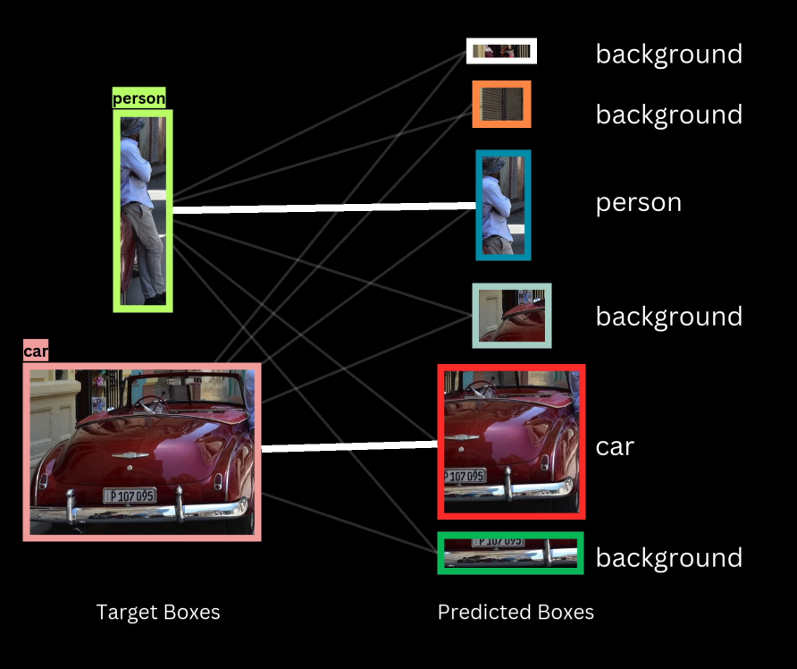
DETR enforces a one-to-one mapping between predicted boxes and ground truth target boxes, ensuring that each target is assigned to a single prediction and each prediction is assigned to a single target or background.
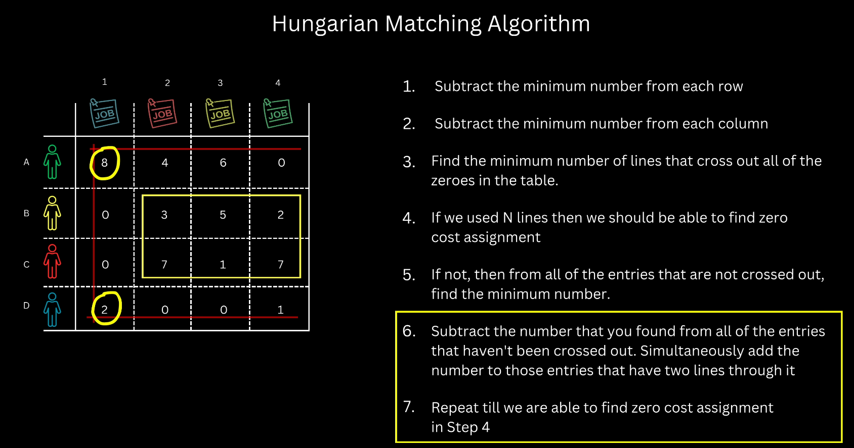
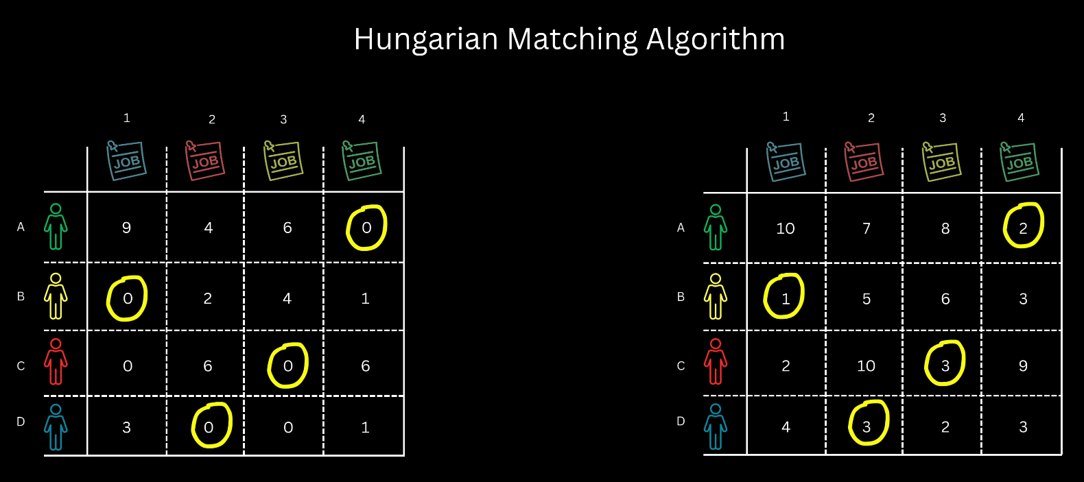
Hungarian Matching Algorithm
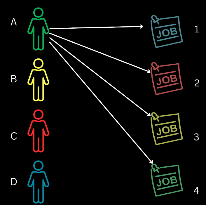
The Hungarian algorithm is employed to find the unique assignment that minimizes the total cost across all assignments for a given image.
This procedure is analogous to finding the minimum cost assignment of $N$ workers to $N$ tasks, requiring a square cost matrix.
Implementation Strategy: To ensure a square matrix, the number of object queries is set to the maximum expected objects in any image (e.g., 100). If targets are fewer than queries, dummy background boxes are conceptually added to the target set; assigning a prediction to a dummy box incurs zero cost.
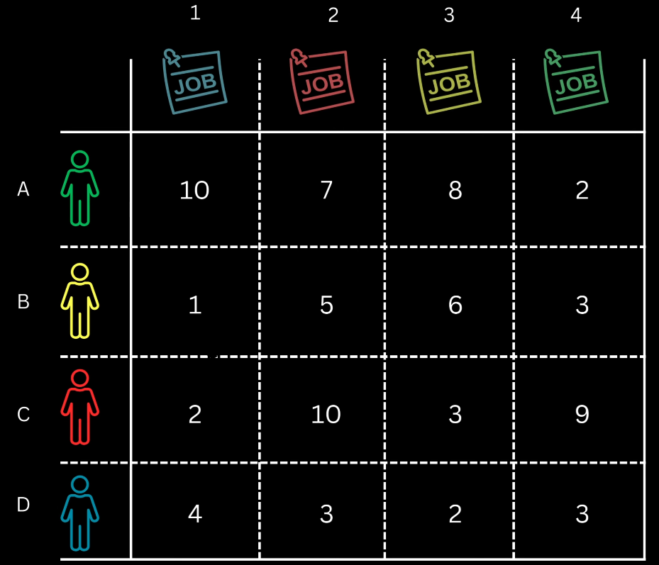
Principle: The core mechanism relies on subtracting or adding a fixed number to all elements in a row or column, which modifies the costs but does not alter the identity of the optimal assignment. The goal is to maximize the number of zero-cost assignments.
Assignment Cost Formulation 
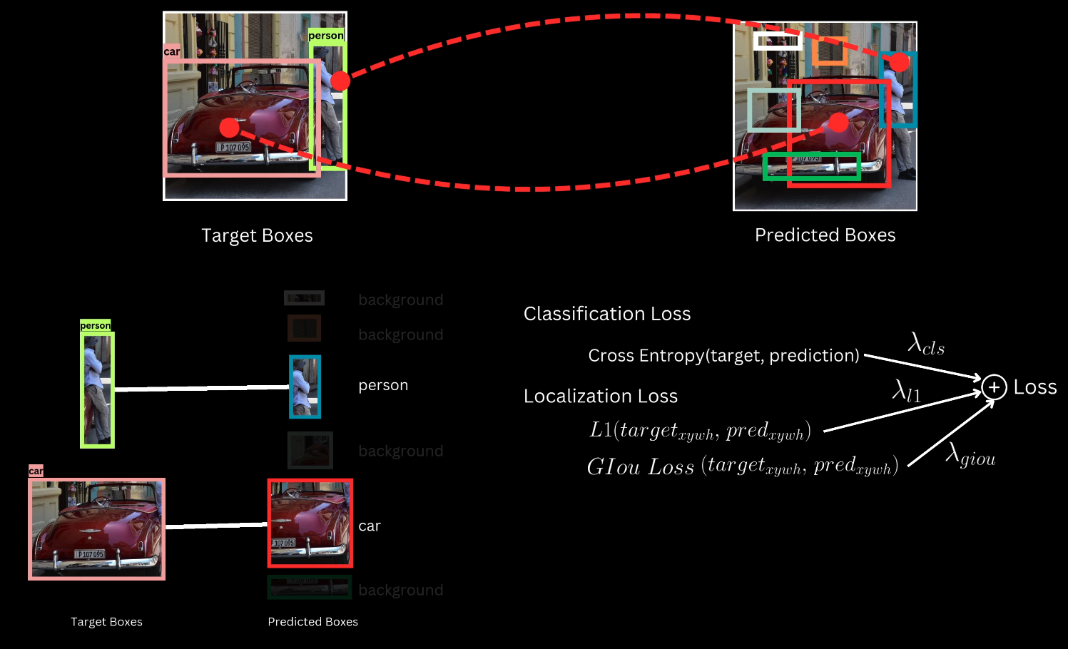
The cost ($\mathcal{C}$) of assigning a predicted box ($p$) to a target box ($t$) is a weighted sum of two primary components: classification cost and localization cost.
Classification Cost: Based on the predicted probability score for the target box’s class label. Since low cost is desired when the probability is high, the cost is calculated as $1 - P_t$, where $P_t$ is the probability predicted for the target class $t$.
Localization Cost: This composite cost measures the closeness of the predicted box to the target box.
L1 Distance: Computed between the normalized coordinates ($c_x, c_y, w, h$) of the target and predicted boxes.
Generalized IOU (GIOU): Used because L1 distance is sensitive to box size differences. To ensure lower cost corresponds to higher overlap, negative Generalized IOU is used.
The total cost for assignment $i$ is:
$$ C_i = \lambda_{cls} \cdot Cost_{cls} + \lambda_{L1} \cdot Cost_{L1} + \lambda_{GIOU} \cdot Cost_{GIOU} $$
DETR Set Prediction Training Loss 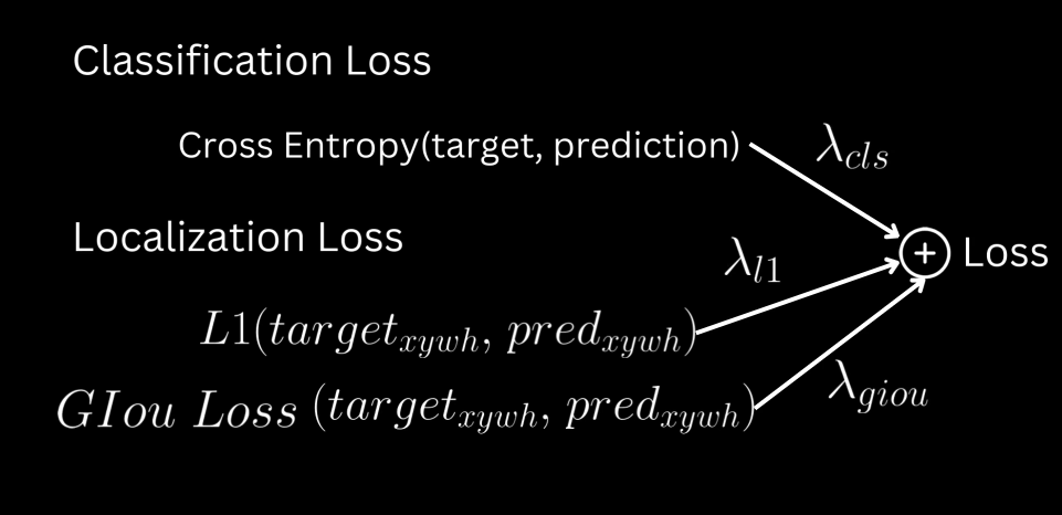
The loss function utilizes the optimal assignment returned by the Hungarian algorithm to drive training. The loss is a weighted sum of classification loss and localization loss.
Classification Loss
- Cross-Entropy Loss is applied between the target class labels and the predicted class probabilities for every box.
- For predicted boxes assigned to a ground truth target, the target label is the assigned target’s class.
- For unassigned boxes, the target label is background.
Localization Loss
Localization loss is computed only for predicted boxes assigned to a non-background class.
The components are:
- Smooth L1 Loss: Applied between the target box coordinates and the predicted box coordinates.
- Generalized IOU Loss (GIOU Loss): Defined as $1 - \text{GIOU}$. Minimizing this loss encourages the model to increase the overlap between the predicted and matched target boxes during training.
Auxiliary Losses
To enhance convergence and improve performance, auxiliary losses are incorporated during training.
Outputs from all decoder layers are utilized, with each layer’s output being passed through the shared class and bounding box MLPs to generate predictions.
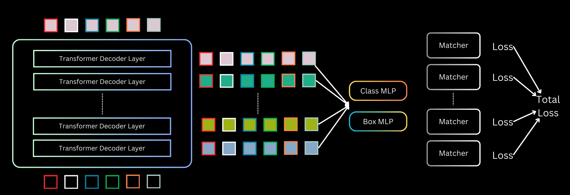
A separate Hungarian matching is performed for the set of predictions generated at each decoder layer.
Classification and localization losses are computed for each layer based on these assignments.
The total loss is the summation of the losses from all decoder layers.
This approach ensures that earlier decoder layers learn useful representations, which the subsequent layers refine. Note that during inference, only the final decoder layer output is used.